-
 VIRA KOSHKINA 27 Jan
generative adversarial models
generative compression
local convergence
adversarial training
MSE loss
GAN

Introduction
Generative Adversarial Networks are notoriously unstable and hard to train. Researchers have to employ a variety of tricks to make the adversarial training converge, constantly battling issues such as mode collapse and training divergence. Fortunately for us, when it comes to Generative Compression Networks (GCN), the adversarial training seems to be on its best behaviour, causing much less trouble. Many tricks that are absolutely necessary for training GANs are not required in the compression pipeline. For example, we never observed a mode collapse, our GCNs train without gradient penalty, we don't need to add noise to our input samples to the decoder, and previous experiments indicate that pre-training of encoder-decoder is not necessary for getting stable discriminator training. In this blog post, we aim to understand how exactly our pipeline differs from standard GANs, what it means in terms of stability and convergence and why traditional GAN techniques are often not applicable.
One obvious difference is that in GCN, by nature of compression, we always have access to the ground truth image that we aim to generate. That allows us to use pixel-wise distortion losses in generator (encoder-decoder) training. In this blog post, follow the paper "Which Training Methods for GANs do actually Converge?" and look at a toy example of GAN. We first examine the conditions of its convergence and then discuss how compression specific loss function impacts convergence.
Convergence of GANs
In terms of game theory, we can think of GAN training as a two-player non-cooperative game. The first player is a generator $$G_\theta(z)$$ with parameters $$\theta$$ that wants to maximize its payoff $$g( \theta, ψ)$$, the second player is a discriminator $$D_ψ(x)$$, with parameters $$ψ$$ that aims to maximize $$d(\theta, ψ)$$. The game is at a Nash equilibrium at $$(\theta^* , ψ^*)$$ when neither player can improve its payoff by changing its parameters slightly. When GAN reaches a Nash equilibrium, we can say that it reached local convergence.
One method to train a GAN is to use a Simultaneous Gradient Descent, which can be thought of as a fixed point algorithm that applies an operator $$F(\theta, ψ)$$ to the parameters of the generator and discriminator $$(\theta, ψ)$$ respectively:
$$F(\theta, ψ) = (\theta, ψ) + h v(\theta, ψ)$$,
where $$h$$ is a learning rate and $$v(\theta, ψ)$$ is the Jacobian of $$L$$, our gradient:
\[
\begin{align}
v(\theta, ψ) =
\begin{bmatrix}
-\nabla_\theta \;L (\theta,ψ) \\
\nabla_ψ \;L(\theta, ψ)
\end{bmatrix}
\end{align}
\]
[2] demonstrates that the convergence near an equilibrium point $$(\theta^* , ψ^*)$$ can be assessed by looking at the spectrum of Jacobian of our update operator $$F_h\;'(\theta, ψ)$$ at the point $$(\theta^* , ψ^*)$$:
- If all eigenvalues have absolute value less than 1, the system converges to $$(\theta^* , ψ^*)$$ with a linear rate (our desired case).
- If there are any eigenvalues with absolute values greater than 1, the system diverges.
- If all eigenvalues have an absolute value equal to 1 (lie on the unit circle), it can be convergent, divergent or neither, but if it is convergent, it will generally converge with a sublinear rate.
For detailed proof of why eigenvalues need to lie in a unit circle, see [4] proposition 4.4.1, page 226. This condition directly translates to the eigenvalues of the Jacobian of the gradient $$v$$:
$$F(\theta, ψ) = (\theta, ψ) + h v(\theta, ψ)$$
$$F\;'(\theta, ψ) = I + h v\;'(\theta, ψ)$$
and therefore, the eigenvalues of the jacobian of our update operator $$F$$ are:
$$λ = I + h \mu$$
where $$\mu$$ are the eigenvalues of the jacobian of the gradient vector field $$v$$. From here, it is trivial to show that for a positive h, $$|λ| < 1$$ is only the case when $$\mu$$ has a negative real part. More specifically:
- If all eigenvalues have negative real-part, the system converges with a linear convergence rate (with a small enough learning rate).
- If there are eigenvalues with positive real-part, the system diverges.
- If all eigenvalues have zero real-part, it can be convergent, divergent or neither, but if it is convergent, it will generally converge with a sublinear rate.
In fact, for a GAN with positive real parts to converge, we would require a negative step size, which is impossible since our $$h$$ is always above 0.
Intuitively we can understand this requirement if we think of GAN updates as a fixed point iteration. Then we can think of the updates as the Euler discretization of the first-order ODE of the gradient vector:
$$\frac{dL(\beta)}{d\beta} = v(L(\beta))$$
Where $$\beta$$ represents our parameters. The Euler step (with step size $$h$$) becomes:
$$\beta^{k+1} = \beta^k + h v(L(\beta))$$
This means that our convergence analysis is, in fact, an analysis of the critical points, nodes and saddle points of the ODE. We can then visualise the behaviour of the system by plotting $$v(\theta, ψ)$$ as a collection of arrows with a given magnitude and direction, each attached to a point $$(\theta, ψ)$$. Figure 1 visually shows how the behaviour of the system changes depending on the eigenvalues of the Jacobian of $$v(\theta, ψ)$$. Subplot c) demonstrates what it means to have negative real values and zero imaginary values, which would be the ideal case for the convergence of our fixed point.
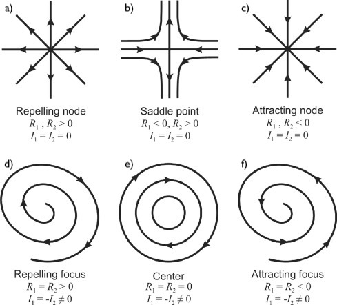 Figure 1. Classification of critical points of a 2D vector field according to eigenvalues. $$R_1$$, $$R_2$$ denote the real parts of the eigenvalues of the Jacobian matrix and $$I_1$$, $$I_2$$ - the imaginary parts. The figure was modified from Figure1 in [5].
Having the criteria for convergence and a tool to visualise the behaviour in a 2D case, we can start the analysis of GAN models. To analyse the behaviour of different training methods and visualise the findings, the authors in [1] propose to look at a toy example called Dirac GAN.
Dirac-GAN
The Dirac-GAN consists of a (univariate) generator distribution $$p_\theta = \delta_\theta$$ and a linear discriminator $$D_ψ(x) = ψ x$$. The true data distribution $$p_D$$ is given by a Dirac-distribution concentrated at 0.
Therefore, under this formulation, both the discriminator and the generator has exactly one parameter. This simplicity allows us to easily plot the vector field for the GAN in a 2D space. For a great explanation of vector fields and convergence of GANs, check out this inFERENCe blogpost.
The non-saturated GAN generator loss is:
$$\max_{\theta}L(\theta , ψ) = f(-ψ \theta)$$
where $$f(t) = - \log (1 + e^{-t})$$. The discriminator loss is:
$$\max_{ψ}L(\theta , ψ) = f(ψ \theta) - const$$
The gradient vector is then:
\[
\begin{align}
v(\theta, ψ) =
\begin{bmatrix}
- ψ f'\;(-ψ \theta) \\
\theta f'\;(ψ \theta)
\end{bmatrix}
\end{align}
\]
The system has a unique equilibrium point of the training objective, at point
$$(\theta, ψ) = (0, 0)$$. Indeed, since $$f(0)=const$$, $$L(\theta , 0) = L(0 , ψ) = const$$ for all $$\theta, ψ \in R$$. Therefore $$(\theta^*, ψ^*) = (0, 0)$$ is a Nash-equilibrium. Now, assuming that $$f(0) \ne 0$$ we have that $$v(\theta, ψ) =0$$ only if $$\theta = ψ = 0$$.
Now we can analyse the convergence of the Dirac-GAN around the equilibrium point $$(\theta^*, ψ^*) = (0, 0)$$ by calculating the Jacobian of the gradient vector field at the equilibrium point:
\[
\begin{align}
v(\theta, ψ) =
\begin{bmatrix}
f'\;'\;(- \theta ψ)ψ^2 & -f' \;(- \theta ψ) \theta ψ + f\;'\;'\;(- \theta ψ)\theta ψ \\
f' \;(\theta ψ) + f'\;' \;(\theta ψ) \theta ψ & f'\;'(\theta ψ)\theta^2
\end{bmatrix}
\end{align}
\],
\[
\begin{align}
v\;'\;(0, 0) =
\begin{bmatrix}
0 &f\;'\;(0)\\
f\;'\;(0) & 0
\end{bmatrix}
\end{align}
\],
which has two eigenvalues, $$± f'(0)i$$, which are both on the imaginary axis. This means that the model is not convergent with a linear rate, as it has zero real parts and we expect to see a circular vector field.
We can visualise the training behaviour of Dirac-GAN by plotting the vector fields for the gradient $$v$$ and the current state of the system. Figure 2 demonstrates the training behaviour of Dirac-GAN with non-saturating GAN loss in the first 500 steps. The left panes show the gradient vector field of Dirac-GAN (arrows) and the current state of the parameters in blue. An error starting at a given point $$(\theta, ψ)$$ shows the value of the gradient $$v(\theta, ψ)$$ at that point. The right panel shows the ground-truth value of the generator parameter $$\theta^* = 0$$ in green and the current value of the learned $$\theta$$ in blue. The orange line represents the angle of the gradient. Dirac GAN with non-saturating loss converges very slowly, with a non-linear rate.

Adding MSE
Above we look at the non-saturating GAN loss, used in standard generative modelling. Now, let us look at what happens once we adapt this to GCN loss, by adding MSE to the loss for the generator parameters $$\theta$$. The discriminator loss stays the same, but the generator loss becomes:
$$\max_{\theta}L(\theta , ψ) = f(-\;ψ \theta) - (0-\;\theta)^2 $$
The gradient vector field now has an additional $$-2 \theta$$ term is the $$\theta$$ partial derivative:
\[
\begin{align}
v(\theta, ψ) =
\begin{bmatrix}
- ψ f'(-ψ \theta) - 2 \theta \\
\theta f'(-ψ \theta)
\end{bmatrix}
\end{align}
\]
The Jacobian of the vector field becomes:
\[
\begin{align}
v\;'(0,0) =
\begin{bmatrix}
- 2 & -f\;'(0)\\
f\;'(0) & 0
\end{bmatrix}
\end{align}
\]
And eigenvalues of the Jacobian of the gradient vector field at the equilibrium point is $$-1 ± \sqrt{1- f'(0)}$$, both of which have negative real parts and 0 imaginary parts, which means that the system should be locally convergent around $$(0,0)$$. The lack of imaginary parts means that there should not be any circular non-convergent behaviour in the gradient vector field. If we now run the Dirac GAN training with this updated generator loss function, we should see convergence and attracting gradient field if the theory matches the practical results. We demonstrate the results in Figure 3.
Figure 3. Training behaviours of Dirac-GAN with the non-saturating loss and added MSE. Left: Vector field and the training state of the system visualise for 500 steps. The starting position is marked in red. Right: Current value of the generator parameter $$\theta$$. The green line indicated the value of the gt parameter $$\theta^* = 0$$, and the blue line shows the estimated $$\theta$$. The orange line shows the current angle of the gradient.

Vanilla GAN loss
We can repeat the analysis for the vanilla GAN loss function. The gradient vector is then:
\[
\begin{align}
v(\theta,ψ) =
\begin{bmatrix}
- ψ f\;'(- ψ\theta)\\
\theta f\;'( - ψ\theta)
\end{bmatrix}
\end{align}
\].
As before, the system has a unique equilibrium point of the training objective at the point $$(\theta^* , ψ^*) = (0, 0)$$.
The Jacobian of the gradient vector field at the equilibrium point:
\[
\begin{align}
v\;'(\theta,ψ) =
\begin{bmatrix}
- f\;'\;'(\theta ψ)ψ^2 & - f\; '(\thetaψ) -f\;'\;'(\thetaψ)\theta ψ\\
f\;'(\theta ψ) + f\;'\;' (\thetaψ)\theta ψ & f\;'\;'(\theta ψ) \theta^2
\end{bmatrix}
\end{align}
\],
\[
\begin{align}
v\;'(0,0) =
\begin{bmatrix}
0 & -f\;'\;(0)\\
f\;'(0) & 0
\end{bmatrix}
\end{align}
\],
which has two eigenvalues, $$± f'(0)i$$, which are both on the imaginary axis. This means that the model is not convergent as it has zero real parts and we expect to see a circular vector field. Figure 4 demonstrates that Dirac-GAN with vanilla GAN loss is divergent around the equilibrium $$(0, 0)$$.
However, for similar reasons as above, the behaviour completely changes once we add the MSE component to the generator loss. The gradient vector field now has an additional $$-2 \theta$$ term in the $$\theta$$ partial derivative:
\[
\begin{align}
v(\theta,ψ) =
\begin{bmatrix}
- ψ f\;'(ψ \theta) - 2\theta\\
\theta f\;' (ψ \theta)
\end{bmatrix}
\end{align}
\],
The Jacobian of the vector field becomes:
\[
\begin{align}
v\;'(0,0) =
\begin{bmatrix}
- 2 & -f\;'(0)\\
f\;'(0) &0
\end{bmatrix}
\end{align}
\],
And, just like in the case of non-saturating loss, eigenvalues of the Jacobian of the gradient vector field at the equilibrium point are $$-1 ± \sqrt{1- f'(0)}$$.

The orange line shows the current angle of the gradient.
This analysis shows that adding MSE has the same impact as gradient regularisation and instance noise, which also remove the circular behaviours in the gradient field and force the negative real part in the eigenvalues. This would explain why these solutions were not impactful when applied to GCNs.
Conclusion
Adding MSE loss for the generator parameter completely changes the training behaviour of the system, making it converge and do it fast. Meaning that MSE loss acts as a regulariser. This can potentially explain why our GCNs, which are always trained with MSE components in the loss, show much better convergence than standard GANs.
References
[1] Mescheder, Lars, Andreas Geiger, and Sebastian Nowozin. "Which training methods for GANs do actually converge?." International conference on machine learning. PMLR, 2018. https://arxiv.org/pdf/1801.04406.pdf
[2] Mescheder, Lars, Sebastian Nowozin, and Andreas Geiger. "The numerics of gans." arXiv preprint arXiv:1705.10461 (2017). https://arxiv.org/pdf/1705.10461.pdf
[3] Huszár Ferenc "GANs are Broken in More than One Way: The Numerics of GANs." https://www.inference.vc/my-notes-on-the-numerics-of-gans/
[4] Bertsekas, Dimitri P. "Nonlinear programming." (1999). https://nms.kcl.ac.uk/osvaldo.simeone/bert.pdf
[5] Theisel, Holger, and Tino Weinkauf. "Vector field metrics based on distance measures of first order critical points." (2002). http://wscg.zcu.cz/wscg2002/Papers_2002/D49.pdf
RELATED BLOGS

 ALEX CHERGANSKI
- 24 Nov


 AARON DEES
- 14 Apr