-
 HAMZA ALAWIYE 19 Apr
A review of Plenoxels: Radiance Fields without Neural Networks
by Hamza Alawiye and Jonathan Rayner
What if we told you that, given several images of a scene from different angles, you can train a model that produces entirely new views of the scene, like this:
Your response is probably either
If you're not impressed yet, how about this: the model that generated this video doesn't use neural networks and is 100 times faster to train than the leading models that do, without sacrificing visual quality.
In this blog post, we review the paper Plenoxels: Radiance Fields without Neural Networks, which describes these innovations. Look how fast the Plenoxels model trains in real time, compared to the standard deep learning alternative NeRF:
The final results are very impressive:
What to expect in this post:
In recent years, there has been a flurry of activity around implicit neural representations of geometric objects. To illustrate with one of the first applications, suppose that we wish to render a 3D shape. Instead of representing it as a discrete grid of volume or surface elements, why not instead represent it as a continuous mapping $$\mathscr{F}$$ from coordinates $$\mathbf{x} = (x, y, z)$$ to a binary occupancy value:
$$\mathscr{F}(\mathbf{x}) = \begin{cases}0 & \mathbf{x}\text{ is outside the shape}, \\ 1 & \text{otherwise}.\end{cases}$$
This is essentially a binary classification problem, which can be solved by any number of machine learning approaches. As suggested by the "neural" in "neural representations", here the function $$\mathscr{F}$$ for a particular shape is parametrised by a neural network. A sufficiently expressive network can capture arbitrarily complex geometry when provided with enough training examples.
It is worth observing that this is somewhat different to the usual application of neural networks (and indeed most other machine learning paradigms): instead of training a single model to perform a general task, we train one neural network per shape that we wish to represent. In some sense, we "overfit" each network so that it captures all of the information within its training data and in doing so learns a continuous representation of a single shape.
View synthesis is a related, more complex task involving rendering new views of an object from arbitrary viewing directions. This requires not only some notion of where the shape is, but also its colour and opacity, both of which could vary according to the viewing direction.
The seminal paper NeRF: Representing Scenes as Neural Radiance Fields for View Synthesis used implicit neural representations to learn mappings from a joint position and viewing direction coordinate $$(\mathbf{x}, \mathbf{d}) \cong (x, y, z, \theta, \phi) \in \mathbb{R}^3 \times \mathbb{S}^2$$ to a scalar optical density and vector RGB colour $$(\sigma, \mathbf{c}) \in \mathbb{R} \times \mathbb{R}^3$$ - a radiance field. The optimisation objective involved using classical volume rendering to determine the colour of a ray passing through the scene in a differentiable manner and simply computing the squared error between the predicted colour and the ground truth.
This approach was shown to be extremely effective, producing high quality renderings from new viewpoints and capturing complex lighting effects. However, the training times are extremely long - on the order of days per scene.
The NeRF paper sparked a surge of further research efforts which extended the model to include features such as re-lighting and background modelling and tried to reduce the runtime costs associated with both training and rendering. Reviewing all of these papers is outside the scope of this blog, but the following two papers had significant influence on Plenoxels:
The Plenoxels paper took a more radical approach by asking the following question:
Is the fundamental advance in NeRF that enabled learned view synthesis the implicit neural representation or the differentiable volume rendering formulation?
Their results show that it is the latter: an equally performant but much simpler model can be fitted using the same optimisation objective as had been used for the neural radiance field approach. The high level overview is that a scene can be represented as a sparse grid of volume elements (voxels), each of which stores coefficients for spherical harmonics that describe changes in colour from different view directions (plenoptic; relating to the light field). These coefficients can be optimised using standard techniques and interpolated between to specify the full radiance field.
We now describe how this works.
The problem of rendering new views of a scene is well studied and has resulted in a number of standard techniques for its solution. Each of these techniques requires the construction of an underlying representation of the three-dimensional geometry of the scene in question.
One such approach is volume rendering, in which data such as colour and optical density (denoted $$\mathbf{c}$$ and $$\sigma$$ respectively) are modelled on a simple three-dimensional volumetric grid rather than attempting to capture the (potentially complex) two-dimensional surface geometry of objects in the scene. Each volume element is typically referred to as a voxel.
Once the voxel grid has been constructed, each scalar field can be extended to fill the entire space by interpolating the values at the voxels. Finally, arbitrary new views can be rendered by volume ray casting.
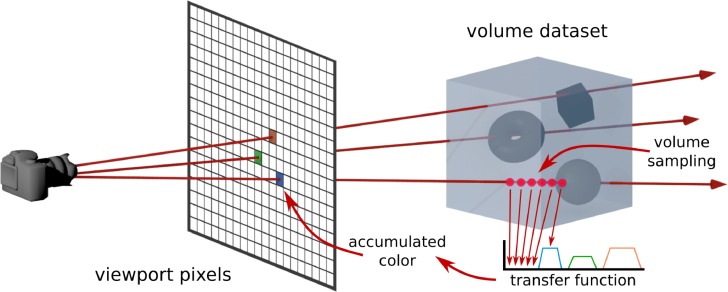 An illustration of Volume Rendering by Ray Casting. In the Plenoxels paper, we only have access to a dataset of 2D views and are attempting to model the underlying 3D structure. The goal is to render new 2D views by tracing out rays from a given view direction. Source.
NeRF and its predecessors, as well as the Plenoxels paper all follow this approach. What's of particular interest is how a simplified model of light interacting with objects lets us set up a useful optimisation problem that solves the task.
In order to establish the colour of a ray of light, one must cast it through the scene and compute the contribution of each point that it passes through to the final observed colour.
So: if a light ray passes through a 3D scene, what colour do we expect to see at our camera?
It turns out that we can obtain a closed form solution to this question, given some simplifying assumptions. To do this, we summarize the well-known paper Optical Models for Direct Volume Rendering, which describes how volume rendering can be achieved with ray casting, using simple ideas from optics (here is a video summary of the idea, if you prefer video).
Imagine that light is passing through an object. As a simplification, we imagine that the interaction is limited to particles absorbing light and/or emitting (or reflecting) some light of their own. We ignore any higher-order effects like shadows and scattering of light between particles, although one can create more complicated models that include these effects.
We can model the absorption of light by the object as the light being obstructed by a collection of identical, opaque, spherical particles with radius $$r$$ . Suppose that the light is passing through a cylindrical volume of length $$\Delta s$$ and cross-sectional area $$E$$:
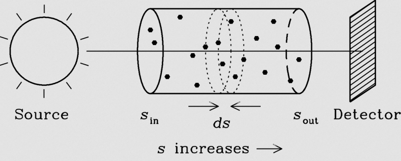 We model light interacting with an object as light interacting with a sparse collection of spherical particles. Here we visualize and infinitestimal cylindrical volume element with height $$ds$$. Source.
If $$\Delta s$$ is sufficiently small, the probability of particles' shadows on the base of the cylinder overlapping is also small, and the area of light occluded is approximately equal to the cross-sectional area of a particle multiplied by the number of particles: $$A \rho E \Delta s$$ (here $$\rho$$ is the particle density ie. number of particles per volume). Thus, the ratio of light blocked to light entering the cylinder is $$A \rho \Delta s$$.
The particles also emit some light, which we assume to be uniform with intensity $$c$$ per unit of cross-sectional area. By the same logic as above, the total contribution to the light emission is $$cA\rho E \Delta s$$.
All together, the change in light passing through the cylindrical volume from absorption and emission is given by
$$\Delta C = c A \rho \Delta s - C A \rho \Delta s ,$$
where $$C$$ is the light intensity entering the volume. For simplicity, we consider light intensity $$C$$ to be a scalar (corresponding to greyscale images), but the calculations readily generalise to colour images by replacing it with a vector intensity for red, green and blue wavelengths.
Let us define the extinction coefficient $$\sigma = A \rho$$ to simplify the expression. We now consider light passing through many of these volume elements of length $$\Delta s$$ and parameterise its path by a variable $$s$$. Taking the limit $$\Delta s \rightarrow 0$$, we obtain
$$\frac{d C}{ds} = \sigma(s)c(s) - \sigma(s)C(s)$$
This differential equation can be solved exactly with an integrating factor. If we take the initial condition $$C(0) = 0,$$ i.e. there is no light entering the scene (only emission and subsequent absorption), the solution is
$$C(s) = \int_{0}^{s} \exp \left( -\int_{t}^s \sigma(u) \text{d}u \right)\sigma(t) c(t) \text{d}t.$$
In order to generalise our model to arbitrary rays, we can parametrise each ray as $$\mathbf{r}(t) = \mathbf{o} + t \mathbf{d}$$ for $$t_n \leq t \leq t_f$$, where $$\mathbf{o}$$ is our coordinate origin and $$\mathbf{d}$$ is our viewing direction. Simultaneously, to extend our calculations to the case of vector RGB colour and to capture specular effects, we replace the single-ray scalar emission intensity $$c(t)$$ with the vector field $$\mathbf{c}(\mathbf{r}(t), \mathbf{d})$$.
$$\mathbf{C}(\mathbf{r}) = \int_{t_n}^{t_f} T(t)\sigma(\mathbf{r}(t))\mathbf{c}(\mathbf{r}(t), \mathbf{d}) \text{d}t$$
where
$$T(t) = \exp \left( -\int_{t_n}^t \sigma(\text{r}(u)) \text{d}u \right).$$
$$T(t)$$ is referred to as the accumulated transmittance along the ray and tells us what proportion of light is transmitted through the ray up to point $$t$$.
Note that the RGB colour $$\mathbf{c}$$ can vary both as a function of position and as a function of viewing direction. In this manner, specular reflection can be captured by the model - the colour of mirror-like surfaces is different depending on the direction from which they are viewed.
Given:
our goal is to learn the parameters that describe the structure of the 3D object in a manner that generalizes to being viewed from any direction.
It turns out that we can use the optics-based accumulated transmittance formula from the previous section to turn our task into an optimisation problem with a differentiable loss function, that can be solved with e.g. Stochastic Gradient Descent.
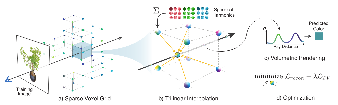 A summary of the Plenoxels approach.
To do this, we approximate the integral expression for $$\mathbf{C}(\mathbf{r})$$ by taking $$N$$ samples $$t_i$$ along the ray and computing the following quadrature:
$$\widehat{\mathbf{C}}(\mathbf{r}) = \sum_{i=1}^N T_i(1 - \exp(-\sigma_i\delta_i))\mathbf{c}_i, $$
where
$$T_i = \exp \left(-\sum_{j=1}^{i-1} \sigma_j\delta_j\right), \quad \delta_k = t_{k+1} - t_k.$$
The key stage in deriving this approximation is the assumption that $$\mathbf{c}$$ is constant between samples (details of this assumption are sorely lacking in many of the papers in the literature). If this is the case, then for a single segment, the following holds
$$\int_{t_i}^{t_{i+1}} T(t)\sigma(\mathbf{r}(t))\mathbf{c}(\mathbf{r}(t), \mathbf{d}) \text{d}t = \int_{t_i}^{t_{i+1}} T(t)\sigma(\mathbf{r}(t))\mathbf{c}_i \text{d}t ,$$
$$= \mathbf{c}_i\int_{t_i}^{t_{i+1}} T(t)\sigma(\mathbf{r}(t)) \text{d}t,$$
$$= \mathbf{c}_i\int_{t_i}^{t_{i+1}} \frac{d}{dt} [T(t)] \text{d}t,$$
$$= \mathbf{c}_i (T(t_{i+1}) - T(t_i)).$$
Replacing the remaining integrals with Riemann sums yields the desired form. Notice that no neural networks are involved!
Side comment: this approximation of the integral makes volume rendering with ray tracing equivalent to alpha compositing (see also this awesome blog post for an introduction to alpha compositing).
At each voxel, the authors store the values of the scalar density and a vector of 9 spherical harmonic coefficients for each colour channel (corresponding to the spherical harmonics of degree $$\leq 2$$).
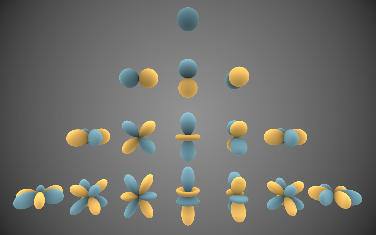 Real spherical harmonics of degree 0,1,2,3 (Inigo Quilez, CC BY-SA 3.0)
The real spherical harmonics $$\{Y_{lm}(\theta, \phi) : l, m \in \mathbb{Z}, l \geq |m|\}$$ are an infinite family of real-valued functions on the sphere. They form an orthogonal basis for square-integrable functions on the sphere in precisely the same way that one can express a function on the circle as a Fourier series expansion. That is to say, just as for any $$g : \mathbb{S}^1 \rightarrow \mathbb{R}$$, we can write
$$ g(\theta) = \sum_{n = -\infty}^{\infty} A_n \exp(i n \theta), $$
or, equivalently,
$$ g(\theta) = \frac{1}{2}a_0 + \sum_{n = 1}^{\infty} a_n \cos( n \theta) + b_n \sin(n \theta), $$
for any $$f : \mathbb{S}^2 \rightarrow \mathbb{R}$$, we can write
$$ f (\theta, \phi) = \sum_{l=0}^{\infty}\sum_{m = -l}^{l} k_{lm} Y_{lm}(\theta, \phi).$$
The colour $$\mathbf{c}_i $$ at a sample point can be computed by summing the spherical harmonics weighted by their coefficients and evaluating the result on the element of $$\mathbb{S}^2$$ corresponding to the viewing direction $$\mathbf{d}$$. I.e. if
$$\mathbf{d} = (\cos \theta \sin \phi, \sin \theta \sin \phi, \cos \phi),$$
then
$$\mathbf{c}_i = \sum_{l=0}^{2}\sum_{m = -l}^{l} k_{lm}^{(i)} Y_{lm}(\theta, \phi).$$
The authors truncate the series expansion at degree $$2$$. Including higher degree harmonics allows higher angular frequencies to be captured, but an ablation study in the PlenOctrees paper showed negligible performance benefits in including harmonics of degree $$3$$ and $$4$$.
Of course, the sample points may not coincide with the locations of the voxels in the voxel grid. The authors compare the use of trilinear interpolation to nearest-neighbour interpolation as methods to construct fields for the density and each spherical harmonic coefficient over the whole volume. They find that the continuously varying field constructed by trilinear interpolation is both siginificantly easier to optimise and more performant than the discontinuous field produced by the nearest-neighbour method.
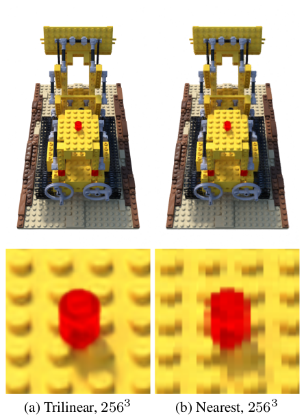 Trilinear interpolation appears to be preferable to nearest neighbor interpolation. For quantitative comparisons, see Table 1 of the Plenoxels paper.
In order to achieve high resolution imaging while not exceeding the memory footprint of a single GPU, the authors employ the voxel pruning method described in the PlenOctrees paper.
First, they start with a dense, low resolution grid and optimise on that before applying a threshold to either the value of $$\sigma_i$$ (a direct threshold on density) or maximal value of $$T_i (1 - \exp(- \sigma_i\delta_i))$$ over all of the training rays (a measure of which voxels are least visible). Voxels below the threshold (the authors do not discuss how they choose this hyperparameter or the thresholding method) are removed and the remaining voxels are divided into 8 before optimising further.
The scheme is further refined by only removing voxels if all of their neighbours are also deemed to be unoccupied: this reduces artifacts around surfaces.
To set up the optimization problem, the authors opt for a mean squared error loss between known images and the images rendered by integrating along rays to obtain $$\widehat{\mathbf{C}}(\mathbf{r})$$. The loss is averaged over batches of rays for a single scene:
$$\mathscr{L} = \frac{1}{ | \mathscr{R} |} \sum_{\mathbf{r} \in \mathscr{R}}|| \mathbf{C}(\mathbf{r}) - \widehat{\mathbf{C}}(\mathbf{r}) ||_2^2$$
Since the view estimate $$\widehat{\mathbf{C}}(\mathbf{r})$$ is differentiable, we can directly optimise the values needed to render images in a given view direction with e.g. gradient descent (in practice the authors use RMSprop - Adam would likely also be fine).
Solving the view synthesis task using volume rendering is an Inverse Problem: It's thus unsurprising that one or more forms of regularization are needed. Here we describe the forms of regularization used.
The authors also find that it's important to include a total variation (TV) regularizer in the loss function, which is defined as:
$$\mathscr{L}_{TV} = \frac{1}{ |\mathscr{V}| } \sum_{\mathbf{v} \in \mathscr{V}, d \in [D]}
\sqrt{\Delta_x^2(\mathbf{v},d) + \Delta_y^2(\mathbf{v},d) + \Delta_z^2(\mathbf{v},d)}$$
where
$$ \Delta_x((i, j, k), d) = \frac{|V_d (i + 1, j, k) - V_d (i, j, k)|}{\frac{256} {D_x}} $$
Here $$D_x$$ is the grid resolution in the $$x$$ dimension, and $$V_d (i, j, k)$$ is the $$d$$th value of voxel $$(i, j, k)$$. The factor of 256 is purely for historical reasons.
TV regularizers are typically used to denoise signals in cases where it's important to maintain the appearance of edges, at the cost of higher computational cost than more simple denoising techniques that might blur edges. In practice, the computational cost of TV regularization is mitigated in this paper by sampling a small percentage of voxels for this term in the loss at each training step.
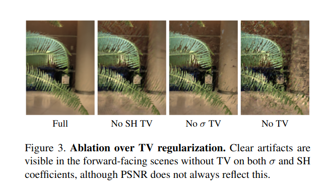
The need for the total variation regularizer is established by Figure 3 of the paper, which shows that the regularizer noticeably removes artifacts that are present at equivalent MSE:
Without pruning the 3D voxel grid, computational costs quickly get out of hand. To do this, voxels with density below a given threshold are pruned throughout training. However, due to the ill-posed nature of the optimization problem, many locations outside of the object's volume can spuriously have density higher than a given threshold and then will never be pruned. This was visualized for exampled in the SNeRG paper:
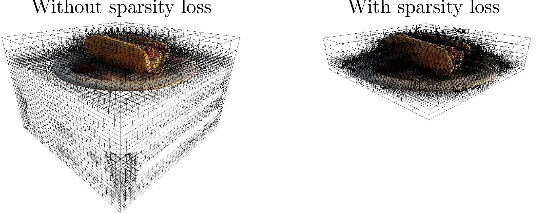 Without a sparsity loss, empty regions can have non-zero density, which greatly adds to computational costs.
Previous work (e.g. SNeRG and PlenOctrees) addressed this by including a regularization term in the loss function to encourage sparsity of the voxel grid. The Plenoxel paper also follows this approach by adding a log Cauchy distribution regularization term:
$$\mathscr{L}_s = \lambda_s \sum_{i,k}\log \biggl(1 + 2\sigma(\mathbf{r}_i(t_k))^2 \biggr)$$
The choice of Cauchy distribution in particular was inspired by the SNeRG paper, but isn't justified further in this paper or in the Plenoxels paper. It's likely that the motivation is to choose a distribution that is fat-tailed and heavily peaked around 0 to encourage sparsity (e.g. Laplace, Cauchy, or $$t$$-distribution). From this point of view it may be that a simple L1 norm on the density would achieve the same goal.
In the case of $$360^{\circ}$$ scenes, an additional regularization term is used to encourage the foreground to either be entirely opaque or empty, which was found to be useful in the Neural Volumes paper. The regularization term is derived as the negative log prior with prior distribution $$\text{Beta} \left(\frac{1}{2}, \frac {1}{2}\right)$$ (also known as the arcsine distribution):
$$\mathscr{L}_{\beta} = \lambda_{\beta}\sum_{\mathbf{r}} (\log(T_{FG}(\mathbf{r})) + \log(1 - T_{FG}(\mathbf{r})) )$$
where $$\mathbf{r}$$ are the training rays and $$T_{FG}(\mathbf{r})$$ is the accumulated foreground transmittance (between 0 and 1) of ray $$\mathbf{r}$$. The motivation for this choice of prior is likely that it is the Jeffreys prior for the probability of success of a Bernoulli trial and since we want the foreground entirely opaque or empty, this is like a Bernoulli trial. By visualizing $$\log(x) + \log(1-x)$$, we can see clearly that the loss is reduced when the opacity in the foreground is either 0 or 1:
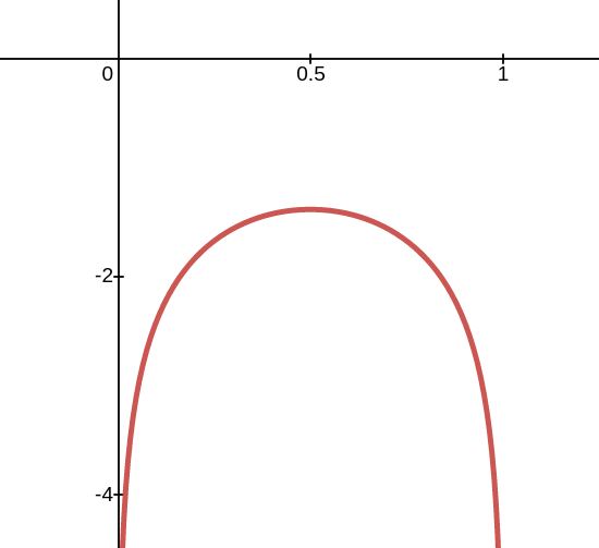 Plot of $$\ln(x) + \ln(1-x)$$. This penalty encourages the opacity to be either 0 or 1 in the foreground.
Okay, that's great and all, but show me what it does!!
Not only are the results on par or better than the existing state of the art, but the training times are extremely quick! The authors train and test the model on 3 different datasets and find excellent results. Let's take a look.
(Remember, all of these videos are the result of training on static 2D images taken from different angles and predicting new unseen views!)
In this task, the Plenoxels is trained on 100 images from different views of synthetic objects. Plenoxels beats NeRF dramatically in terms of training time and quality:
Another example:
Having fun yet? Here are some models that were trained for ~1 minute 20 seconds:
What about more complex scenes? In this task Plenoxels is trained on 20 to 60 forward-facing images captured by a handheld cell phone with resolution 1008 × 756. The resulting videos are impressive:
The next level of difficulty is real unbounded scenes with $$360^{\circ}$$ viewing possibility.
The authors find that they need to make a minor addition to the Plenoxels model to handle the unboundedness of the scene, which they call a "multi-sphere image (MSI) background mode". Essentially the background is learned as a nested collection of concentric spheres with a separate deformed grid from the foreground object grid used thus far. Describing this further is a bit beyond the scope of what we're hoping to convey with this post (see the Plenoxels paper and the NeRF++ paper for more details).
Here's an impressive result from this task:
Here's an awesome example of how the foreground and background can be decomposed in inference using this approach:
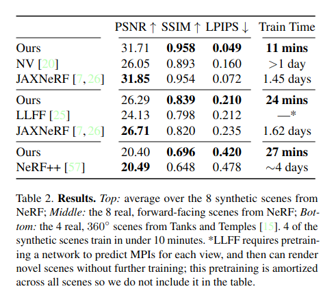
The authors share some impressive quantitative results. Plenoxels either beats or is within striking distance of other existing approaches in term of basic metrics of visual quality, with several orders of magnitude faster training:
Here some things that we think are really cool about this paper:
 ARSALAN ZAFAR
 HAMZA ALAWIYE